Simplified self-attention

Self-attention is like asking: given an input sequence of words, what can I do to selectively compress that sentence into units, where each unit compresses the entire meaning of the sentence by a ratio determined by the relevance of each word to every other word?

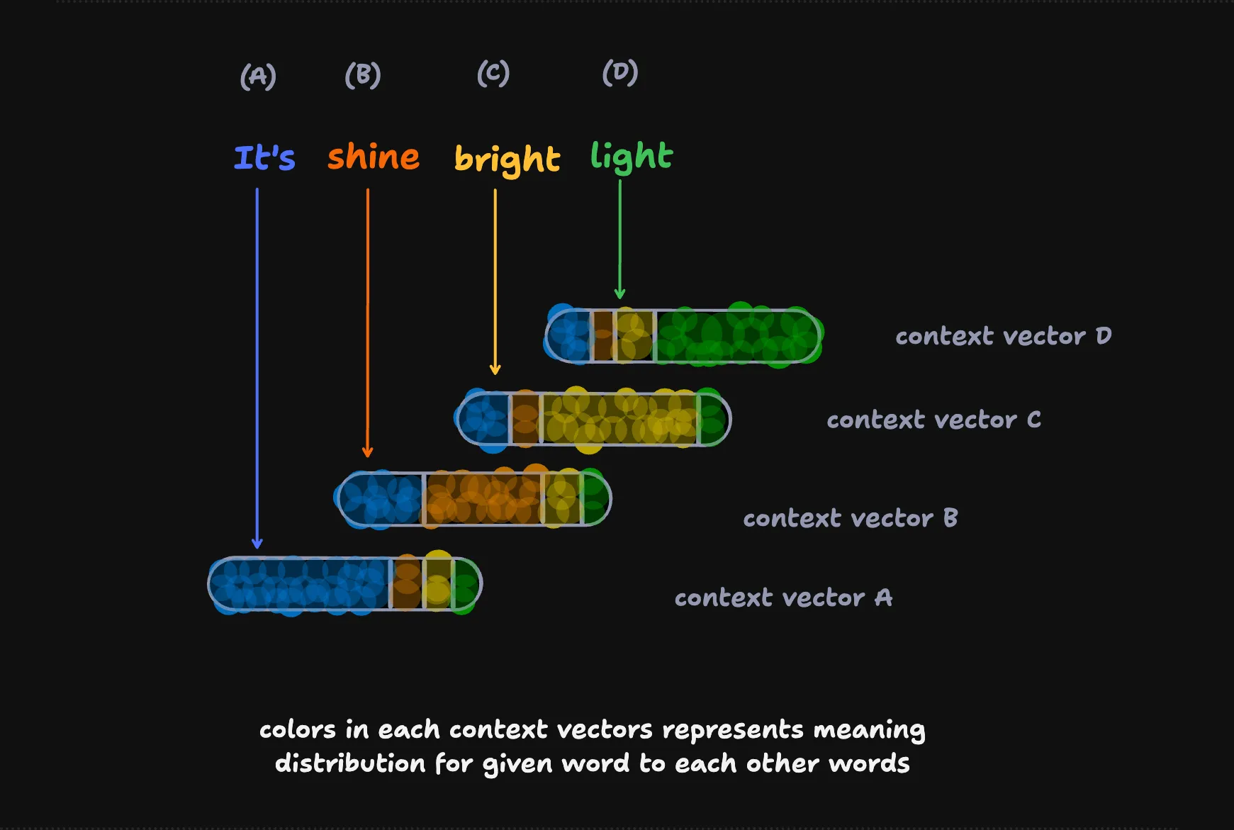
These units form a context matrix, where each row is a context vector: a transformation of the original embedding of that word into a richer, more informed representation. Each context vector is a bird’s-eye view of the entire input sequence, seen through the lens of one specific word.

So the essence of self-attention is creating an attention matrix, and at its core it boils down to a set of matrix operations on the input sequence. We are going to discuss these in detail in this section: dot-product scores between tokens, a softmax to turn them into weights, and a weighted sum to produce context vectors. Then, in the follow-up section, we’ll introduce trainable weights.

Self-attention mechanism step by step

Let’s walk the whole mechanism on one short sentence, It's a shine bright light, using tiny 4-dimensional embeddings so every number stays checkable by hand. In this simplified version there are no trainable weights yet: each token acts as its own query, key, and value.

The core idea

Every token looks at every other token, then rebuilds itself as a weighted blend of the whole sequence.

Step 0: Tokenize

We split the sentence into five word-level tokens, each with an id.

Position	Token	Id
1	It's	1001
2	a	1002
3	shine	1003
4	bright	1004
5	light	1005

Step 1: Embed each token

Every token becomes a row of numbers. Real models use thousands of dimensions; we use four so the matrix fits on the page. This is our embedding matrix X (shape [5, 4]).

Token	d1	d2	d3	d4
It's	1	0	1	0
a	0	1	0	1
shine	1	1	0	0
bright	0	0	1	1
light	1	0	0	1

Step 2: Score every pair (dot products)

To score every pair at once, we multiply our input matrix X by its own transpose Xᵀ. The result is a matrix of numerical values, where each value represents the similarity between one word and every other word in the input.

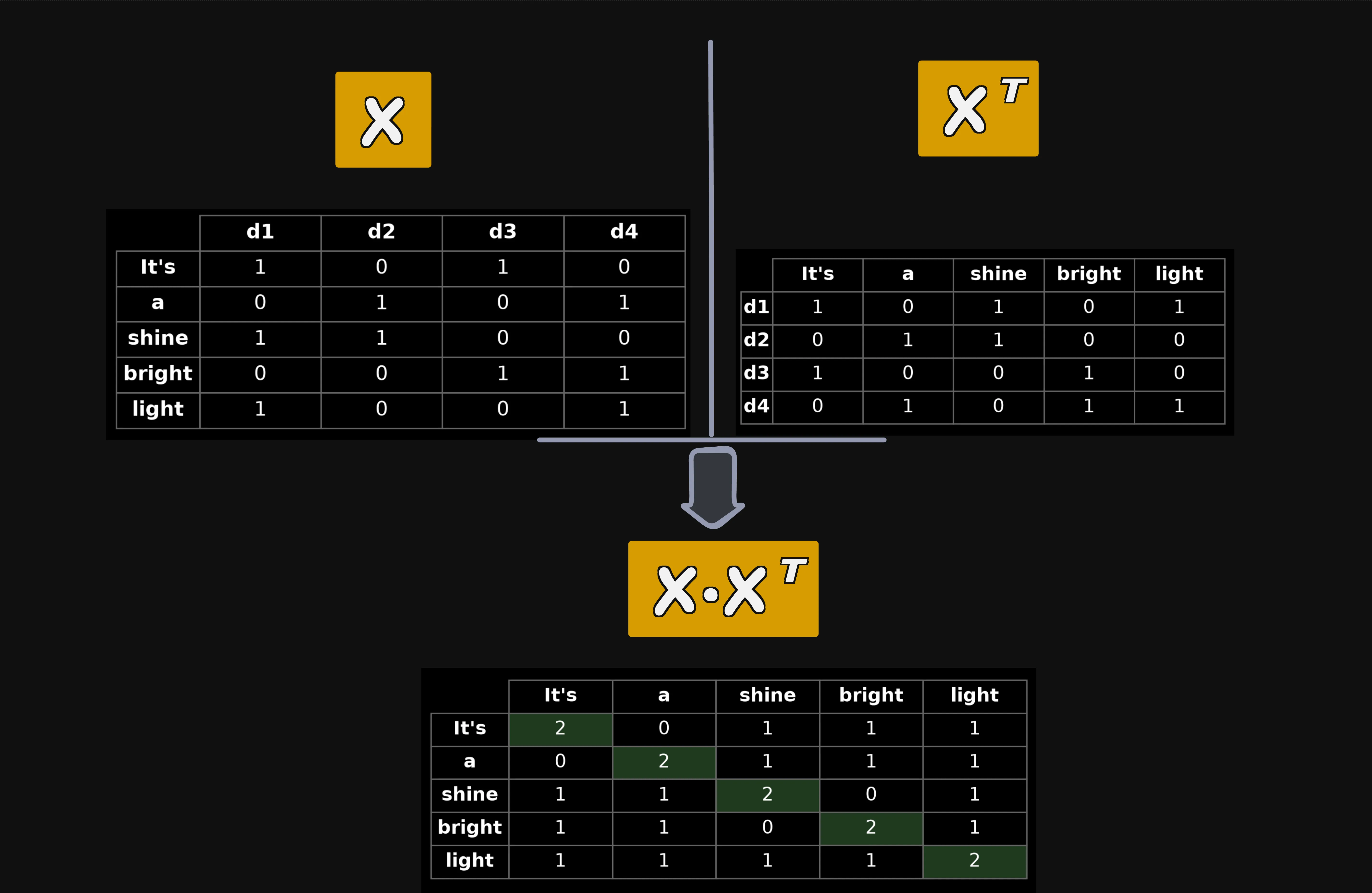
The attention score between two tokens is the dot product of their rows. A larger score means the two tokens are more related. Computing this for every pair gives a [5, 5] score matrix (X · Xᵀ).

Query ＼ Key	It’s	a	shine	bright	light
It’s	2	0	1	1	1
a	0	2	1	1	1
shine	1	1	2	0	1
bright	1	1	0	2	1
light	1	1	1	1	2

In code, we first lay out the five embeddings as a [5, 4] tensor, then multiply it by its own transpose. The true flag transposes the second operand.

import * as tf from "@tensorflow/tfjs-node";

// Our five token embeddings, shape [5, 4].
const X = tf.tensor2d([
  [1, 0, 1, 0], // It's
  [0, 1, 0, 1], // a
  [1, 1, 0, 0], // shine
  [0, 0, 1, 1], // bright
  [1, 0, 0, 1], // light
]);

// Score every pair: X · Xᵀ, shape [5, 5].
const scores = tf.matMul(X, X, false, true);
scores.print();
// [[2, 0, 1, 1, 1],
//  [0, 2, 1, 1, 1],
//  [1, 1, 2, 0, 1],
//  [1, 1, 0, 2, 1],
//  [1, 1, 1, 1, 2]]

Step 3: Scale the scores

We divide every score by the square root of the embedding dimension (√4 = 2). This keeps the numbers in a stable range so the next step behaves well.

Query ＼ Key	It’s	a	shine	bright	light
It’s	1.0	0.0	0.5	0.5	0.5
a	0.0	1.0	0.5	0.5	0.5
shine	0.5	0.5	1.0	0.0	0.5
bright	0.5	0.5	0.0	1.0	0.5
light	0.5	0.5	0.5	0.5	1.0

We read the embedding dimension straight off the tensor shape, then divide by its square root.

// dK is the embedding dimension, 4. We scale by its square root.
const dK = X.shape[1];
const scaled = scores.div(Math.sqrt(dK));
scaled.print();
// [[1.0, 0.0, 0.5, 0.5, 0.5],
//  [0.0, 1.0, 0.5, 0.5, 0.5],
//  ...]

Step 4: Softmax into attention weights

Softmax turns each row of scores into positive weights that sum to 1. Now each row tells us how much a token should draw from every other token. This is the matrix you would draw as a heatmap.

Query ＼ Key	It’s	a	shine	bright	light
It’s	0.314	0.115	0.190	0.190	0.190
a	0.115	0.314	0.190	0.190	0.190
shine	0.190	0.190	0.314	0.115	0.190
bright	0.190	0.190	0.115	0.314	0.190
light	0.177	0.177	0.177	0.177	0.292

Softmax runs over the last axis (-1), so each row is normalized independently.

// Softmax over the last axis: each row becomes weights that sum to 1.
const weights = tf.softmax(scaled, -1);
weights.print();
// [[0.314, 0.115, 0.190, 0.190, 0.190],
//  ...]

Step 5: Blend into context vectors

Finally we use each row of weights to take a weighted sum of the value rows (Z = A · X). The result is a new [5, 4] matrix where every token has been rewritten as a blend of the whole sentence.

Token	z1	z2	z3	z4
It's	0.694	0.305	0.504	0.495
a	0.495	0.504	0.305	0.694
shine	0.694	0.504	0.305	0.495
bright	0.495	0.305	0.504	0.694
light	0.646	0.354	0.354	0.646

One last matrix multiply blends the value rows into the context matrix.

// Weighted sum of the value rows: weights · X, shape [5, 4].
const context = tf.matMul(weights, X);
context.print();
// [[0.694, 0.305, 0.504, 0.495],
//  ...]

Full implementation

The snippets above use plain [5, 4] matrices to keep the numbers readable. The complete SimplifiedAttention class lives in @node-llm/core at packages/core/src/model/attention/simplifiedAttention.ts, where it operates on batched [batch, seqLen, dIn] tensors. You can run the full walkthrough with pnpm ch03:1, source at packages/chapters/src/ch03-attention/01-simplified-attention.ts.

Following one token all the way through

To make the flow concrete, here is the full path for the query It's:

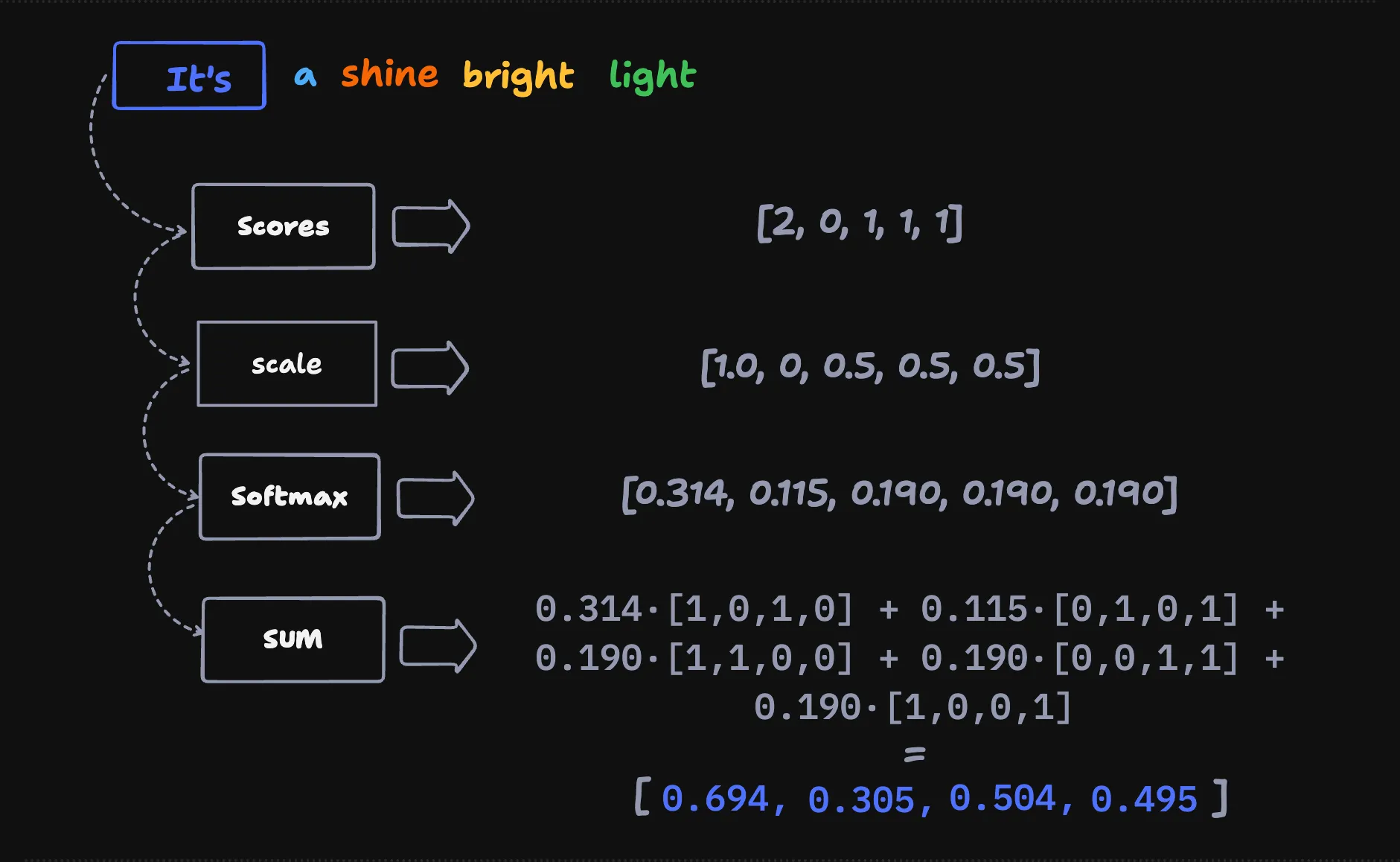
1. Scores against every token: [2, 0, 1, 1, 1]
2. Scale (divide by 2): [1.0, 0, 0.5, 0.5, 0.5]
3. Softmax: [0.314, 0.115, 0.190, 0.190, 0.190]
4. Blend the value rows: 0.314·[1,0,1,0] + 0.115·[0,1,0,1] + 0.190·[1,1,0,0] + 0.190·[0,0,1,1] + 0.190·[1,0,0,1] = [0.694, 0.305, 0.504, 0.495]

And that is the entire mechanism. We take one query, score it against all five keys, run a softmax, and take a weighted sum of the five value vectors to land on a single context vector. In the next lesson we add the trainable Wq, Wk, and Wv projections, and everything should come through exactly the same way.