Self-attention with trainable weights

Everything we’ve done so far with self-attention applies here, and I mean everything. We are not starting over, we are building on top of what we already have. Every step from simplified self-attention carries forward.

The most notable difference in this section is the introduction of three new matrices: Wq, Wk, and Wv.

The key upgrade

These three matrices are what make self-attention trainable. They get updated as the model learns.

Now here is the important thing to understand about where they come from. Wq, Wk, and Wv are projections of the input matrix X, which means they all start from the same place, with the same values. But as training progresses, each one begins to specialize. Each one starts to resemble something useful for its specific job.

• Wq becomes optimized to help produce better query vectors: sharper questions.
• Wk becomes optimized to help tokens better advertise themselves, to surface what is relevant about them when others come looking.
• Wv becomes optimized to yield better values: richer, more meaningful content to pass forward once attention has decided what to focus on.

From input to Q, K, V

We take the same input matrix X and multiply it by each projection matrix. This produces three new matrices: the queries Q, the keys K, and the values V.

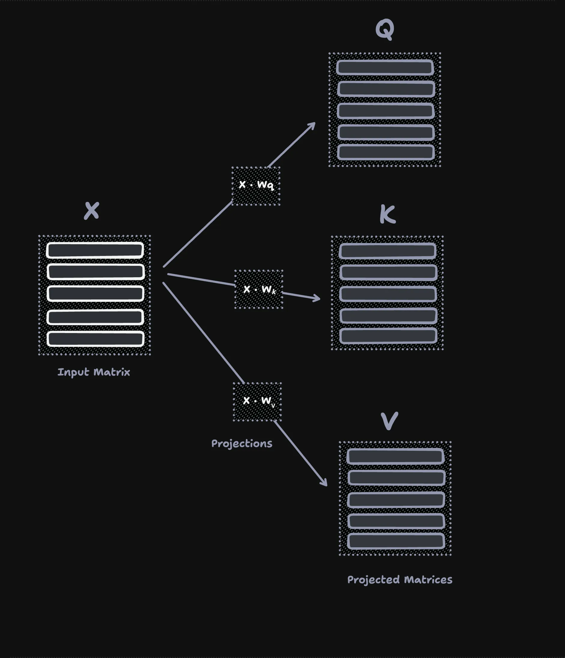
From here, the steps are exactly the ones we used in simplified attention. The only thing that changed is what we feed into them.

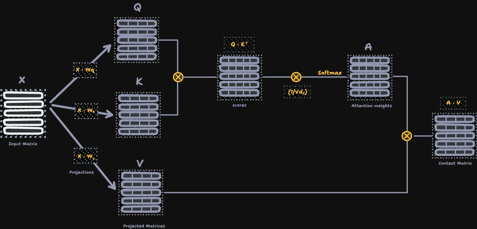
In the previous lesson we worked directly with the raw embeddings X. We took dot products to see how related every pair of tokens was, passed those numbers through softmax to turn them into weights, and built each context vector as a weighted average of the embeddings.

We run those same three steps here, just on our learned matrices instead of on X. Q and K give us the relatedness between tokens, and V provides the vectors we average together into the context vectors.

Here is the full path in one picture, from the input matrix all the way to the context matrix:

In code

First the setup: the same five embeddings, plus the three trainable projection matrices. We wrap each one in tf.variable so the training loop can update it.

import * as tf from "@tensorflow/tfjs-node";

// The same five token embeddings, shape [5, 4].
const X = tf.tensor2d([
  [1, 0, 1, 0], // It's
  [0, 1, 0, 1], // a
  [1, 1, 0, 0], // shine
  [0, 0, 1, 1], // bright
  [1, 0, 0, 1], // light
]);

const dIn = 4; // embedding dimension
const dOut = 4; // attention output dimension

// The trainable projection matrices. They start random, then get optimized during training.
const Wq = tf.variable(tf.randomNormal([dIn, dOut]));
const Wk = tf.variable(tf.randomNormal([dIn, dOut]));
const Wv = tf.variable(tf.randomNormal([dIn, dOut]));

Now we project X into queries, keys, and values, then run the exact same scaled dot-product attention as before.

// Project the input into queries, keys, and values, each shape [5, 4].
const Q = tf.matMul(X, Wq);
const K = tf.matMul(X, Wk);
const V = tf.matMul(X, Wv);

// Scaled dot-product attention, identical to the simplified lesson, but on Q, K, V.
const scores = tf.div(tf.matMul(Q, K, false, true), Math.sqrt(dOut)); // [5, 5]
const weights = tf.softmax(scores, -1); // each row sums to 1
const context = tf.matMul(weights, V); // [5, 4]
context.print();

The shape flow is identical to simplified attention ([5, 5] scores, [5, 4] context). The only difference is that we learn Q, K, and V first instead of scoring the raw embeddings directly.

Full implementation

The snippets above use plain [5, 4] matrices and fresh random weights to keep things readable. The complete SelfAttention class lives in @node-llm/core at packages/core/src/model/attention/selfAttention.ts, where it operates on batched [batch, seqLen, dIn] tensors, tracks its weights for training, and supports an optional causal mask. You can run the full walkthrough with pnpm ch03:2, whose source is at packages/chapters/src/ch03-attention/02-self-attention.ts.

Projection dimensions

Let’s discuss the idea of projections a little more. As we mentioned, they are the same input matrix looked at from different perspectives. A projection can follow the input dimension, or it can compress into a smaller dimension than the input.

Think of it this way. This shows that the attention mechanism can compress or transform the data into an entirely new dimension to look for specific patterns, rather than just copying the original [5, 4] shape.

In our example we have an input matrix of [5, 4] shape, where:

• 5 = the sequence length (rows), and it stays fixed. We always get one context vector per token.
• 4 = the feature dimension (columns), and this is what a projection can change.

Then we matched the projection dimension (dOut) with the input dimension (dIn = 4), so our output kept the same [5, 4] shape. But nothing forces that, we could project into a different dimension. Keep this in mind as we move to the next lesson on multi-head attention, because it will be one of the key ideas.

PyTorch → JS mapping

Reference (Python)	Here (TypeScript)
nn.Parameter(torch.rand(d_in, d_out))	tf.variable(tf.randomNormal([dIn, dOut]))
queries = x @ W_query	tf.matMul(x, Wq)
queries @ keys.T	tf.matMul(q, k, false, true)
scores / keys.shape[-1] ** 0.5	tf.div(scores, Math.sqrt(dOut))
torch.softmax(scores, dim=-1)	tf.softmax(scores, -1)
attn_weights @ values	tf.matMul(weights, v)