A mini neural network layer

Before we build GPT, we need to be comfortable with the smallest piece it is made of. Everything in the model, including attention, is built out of this one idea.

Before we dive into the GPT model architecture, let’s step back a little and talk about a simple neural network layer. Let’s call it a mini layer.

Our mini layer is small on purpose: an input row, then two layers holding three neurons in total, two in the first layer and one in the second. Understanding this will make the more complex blocks of GPT much easier to follow when we get to them in the next sections.

So what is a neural network layer?

A neural network layer is a small machine that takes in numbers, the embedding representation of a token, and produces a new row of numbers using its own weights.

Here is our mini layer, with a second layer stacked after it so we can see where the numbers go next.

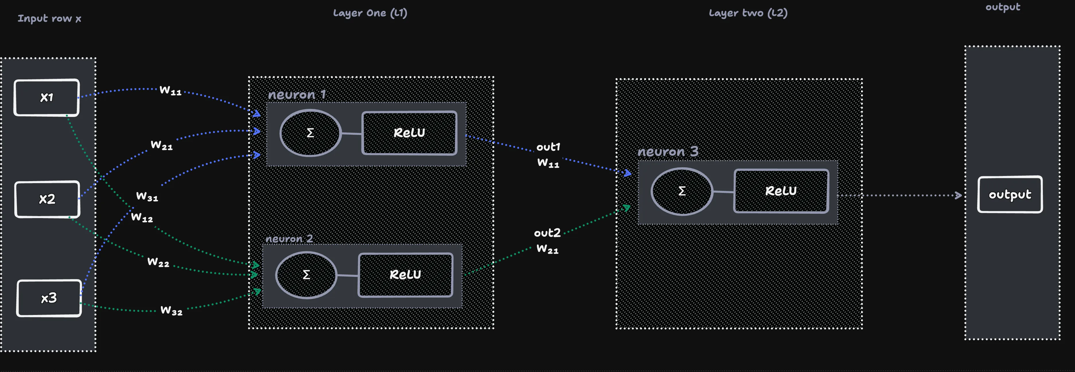
A few things to read off the diagram:

• x1, x2, x3 are not three tokens. They are three features of one token, so they are one row.
• The labels on the arrows are the weights. We write them as w(input, neuron), so w₃₁ is the weight from input 3 into neuron 1.
• Inside every neuron there are two stages: Σ adds things up, then ReLU squashes the result.
• Layer two works exactly like the layer before it. The output of the previous layer becomes its input, and it brings its own trainable weights, which is why its labels start over at w₁₁ and w₂₁. That is the shape of a neural network: a collection of layers repeating the same operation over and over, until we reach the final layer.

What each neuron computes

Every neuron follows the same four steps. Multiply each input by its own weight, add them up, add a bias, then apply ReLU.

out₁ = ReLU(w₁₁·x₁ + w₂₁·x₂ + w₃₁·x₃ + b₁)
out₂ = ReLU(w₁₂·x₁ + w₂₂·x₂ + w₃₂·x₃ + b₂)

The whole recipe

Every neuron does the same thing: multiply each input by its own weight, add them up, add a bias, then squash the result.

The bias is one extra number per neuron that gets added at the end. The diagram leaves those arrows out so it stays readable, but they are always there.

Let’s run real numbers through it with x = [1, 2, 3].

Neuron	Weights	Bias	Weighted sum	After ReLU
1	[0.5, -1, 0.5]	0.1	0.5 - 2 + 1.5 + 0.1 = 0.1	0.1
2	[-1, 0, -0.5]	0	-1 + 0 - 1.5 = -2.5	0

So the output row is [0.1, 0]. Notice that neuron 2 produced a negative sum, and ReLU turned it into a flat zero. This is why layer outputs are often full of zeros.

Neurons are not parameters

These two get mixed up easily, so it is worth separating them.

• Neurons are the circles. Each one produces exactly one output number. Two neurons means two numbers in the output row.
• Parameters are the numbers the model learns: every weight on an arrow, plus one bias per neuron.

In our mini layer there are 3 × 2 = 6 weights and 2 biases, so 8 parameters in total. The number of neurons is a choice we make.

The same weights run for every row

A layer does not keep a separate set of weights per token. It keeps one set, and every row runs through it independently.

That is what decides the shapes:

Tensor	Shape	Meaning
x	[1, 3]	one token, three features
W	[3, 2]	three inputs, two neurons
out	[1, 2]	one token, two features

Feed in five tokens instead of one and the input becomes [5, 3], the output becomes [5, 2], and W does not change at all. The token count stays the same, and only the feature count changes.

By now you might be wondering that each token passing through the neural network has no understanding of the tokens around it. You would be right. A neural network layer lacks the situational context of the input, because every row is processed on its own.

This is exactly why we have the attention block. Attention shares the contextual meaning among tokens, as we discussed in the previous chapter, and that is precisely where it fits in. In the follow-up sections we will refine our model and add the attention mechanism to it.

ReLU, and why it is not a layer

ReLU is the squash step at the end of the recipe, and the rule is as simple as it looks.

ReLU(x) = x if x is positive, otherwise 0

It has no weights and nothing to learn. It is an operation applied to each number on its own, not a layer. People often call it a layer because that is how frameworks expose it, but there are no parameters inside it.

So why do we need it at all? Because without it, stacking layers would be pointless. Two weighted sums back to back collapse into a single weighted sum, since multiplying two matrices just gives you another matrix. The squash in the middle is what lets a deep stack compute something a single layer cannot.

GELU is coming

GPT does not use ReLU. It uses GELU, a smoother version of the same idea. We will build it in the next lesson.

Where the loss lives

We have said a few times now that a neural network has one big equation at its heart. This is the moment to see it.

Each neuron carries a small equation of its own. Our mini network has three of them, two in the first layer and one in the second:

out₁ = ReLU(w₁₁·x₁ + w₂₁·x₂ + w₃₁·x₃ + b₁)
out₂ = ReLU(w₁₂·x₁ + w₂₂·x₂ + w₃₂·x₃ + b₂)
ŷ    = ReLU(w′₁₁·out₁ + w′₂₁·out₂ + b′₁)

The prime is just our way of saying these are layer two’s weights, since the diagram starts its labels over at w₁₁.

Now plug the first two lines into the third, and the whole network folds into a single equation:

ŷ = ReLU( w′₁₁·ReLU(w₁₁·x₁ + w₂₁·x₂ + w₃₁·x₃ + b₁)
        + w′₂₁·ReLU(w₁₂·x₁ + w₂₂·x₂ + w₃₂·x₃ + b₂)
        + b′₁ )

This is the point of the whole thing. No matter how many layers we stack, we always end up with one unified equation that takes the input and produces a single output, ŷ. The network is that equation, and every weight and bias inside it is a knob we are allowed to turn.

But knowing what the network produced is only half of the story. We also know what it should have produced, the target y. Measuring how far ŷ sits from y is what we call the loss function, the holy grail of machine learning:

loss = (ŷ - y)²

That is the simplest form of it, the squared error. GPT uses cross-entropy instead, which we will build in Chapter 5, but the idea is the same in both.

So what is training, in the end? It is nothing more than this: we keep adjusting the knobs of the unified equation so the difference between its output and the target collapses toward zero. One thing to notice about the loss is where it sits. It lives outside every layer, at the very end, and yet it is the number that decides how the weights inside all of them get updated at once.

The loss measures, it does not adjust

The loss tells us how wrong the network is. It does not tell us which way to turn each knob. That job belongs to the gradient, the derivative of the loss with respect to each weight, and backpropagation is what computes it by walking the unified equation backwards. More on that in Chapter 5.

In this lesson there is no training and no loss. We create a layer with known weights, push a row through it, and look at the numbers that come out. That is enough to see what a layer actually does.

In code

The whole mini layer is three tfjs calls. One matMul handles both neurons at once, because each column of W is one neuron’s weights.

import * as tf from "@tensorflow/tfjs-node";

// One input row with three features, shape [1, 3].
const x = tf.tensor2d([[1, 2, 3]]);

// Layer 1: three inputs, two neurons. Each column of W is one neuron.
const w1 = tf.tensor2d([
  [0.5, -1.0], // weights leaving x1, to neuron 1 and neuron 2
  [-1.0, 0.0], // leaving x2
  [0.5, -0.5], // leaving x3
]);
const b1 = tf.tensor1d([0.1, 0.0]);

// The recipe: weighted sum, add the bias, then squash.
const out = tf.relu(tf.add(tf.matMul(x, w1), b1));
out.print(); // [[0.1, 0]]

// Layer 2: two inputs, one neuron, with its own weights.
const w2 = tf.tensor2d([[1.0], [2.0]]);
const b2 = tf.tensor1d([0.0]);

const output = tf.relu(tf.add(tf.matMul(out, w2), b2));
output.print(); // [[0.1]]

The tf.add broadcasts the bias across every row, so the same two bias numbers get applied to each token.

Full implementation

You have already shipped this operation. The project helper in @node-llm/core at packages/core/src/model/attention/utils.ts is exactly this weighted sum plus optional bias, and it is what Wq, Wk, and Wv use under the hood.

PyTorch → JS mapping

Reference (Python)	Here (TypeScript)
nn.Linear(3, 2)	tf.matMul(x, w) then tf.add(..., b)
nn.ReLU()	tf.relu(x)
nn.Sequential(nn.Linear(3, 2), nn.ReLU())	compose the calls directly
layer(x)	layer.forward(x)
torch.rand(2, 5)	tf.randomUniform([2, 5])
out.shape	out.shape

Stacking layers

Layer two treats layer one’s output row as its input. Nothing new happens conceptually, it is the same recipe again with its own weights:

output = ReLU(w₁₁·out₁ + w₂₁·out₂ + b₁)

Our row goes [1, 3] into layer one, comes out [1, 2], then goes into layer two and comes out [1, 1].

And here is the problem that the rest of this chapter exists to solve. Every layer multiplies and adds, so whatever scaling a layer applies gets compounded by the next one.

Scale factor per layer	After 10 layers
1.5 (grows a little)	about 58× bigger
0.7 (shrinks a little)	about 0.03×, almost zero

Numbers that blow up or vanish make training unstable. Now picture a real GPT with dozens of these layers stacked on top of each other, and you can see how quickly a small drift becomes fatal. That is exactly what layer normalization is built to control, and it is where we go next.

Recap

• A layer is a set of weights plus one recipe: weighted sum, add a bias, squash.
• Neurons are the outputs. Weights and biases are the parameters the model learns.
• One set of weights serves every row, so the token count never changes and only the feature count does.
• Stacking layers compounds any change in scale, and that drift is what layer normalization fixes.

Next up: LayerNorm and the GELU feed-forward, the two pieces that keep a deep stack stable.